Magnetic examples: Ce³⁺, Pr³⁺ and OH#

Calculate spin–orbit levels with MPPT2, then g tensors, magnetization and magnetic susceptibility with the magnetic-moment operator at zeroth order in the MPPT perturbation, projected into the retained MPPT2 states.

Example	Demonstrates	Time
Ce³⁺	4f/5d levels and magnetic response	52 min 49 s
Pr³⁺	A multistate 4f²/4f5d reference and susceptibility	2 h 44 min
OH	Molecular spin–orbit splitting and comparison with QDNEVPT2 and coupled cluster	1 h 5 min 27 s

Times sum successful scientific stages on an Intel Core i7-11700 with eight threads. The inputs are in test_suite/workflows/magnetic/ce, pr and oh.

Calculation workflow#

PySCF prepares state-averaged CASSCF orbitals. CIPSIXX selects the model space; DIAGPT constructs the MPPT2 effective Hamiltonian, and HEFFSO calculates spin–orbit states and their magnetic response.

Ce and Pr use density fitting; OH uses exact integrals. All examples use selected-orbital export and spin-projection closure. The selection target counts rows after closure; the number of physical selected determinants is reported separately below.

All three inputs set spin_g: 2.0. See Magnetic Properties for the model, formulas and units. Dashed magnetic curves use the analytic Curie references; each example specifies its comparison manifold and temperature range. On narrow screens, scroll figures horizontally to read their labels.

Ce³⁺: 4f and 5d levels#

Use CAS(1,12) over 4f/5d, averaging 12 doublet states. Selection uses 20 orbitals, full MOs 10–29, including 5s/5p and projected 6s/6p orbitals. The basis contraction is (10s9p9d7f3g2h) → [4s5p5d5f3g2h]: 128 spherical functions, with a 28-electron ECP.

Input and run#

Ce-df-topk20000.yaml is the complete calculation input; Ce_expt_so_with_gh.bas contains the basis and ECP.

ce/Ce-df-topk20000.yaml#

molecule:
  symmetry: false
  charge: 3
  so: true
  max_memory: 16GB
  atoms:
    - [Ce, 0.0, 0.0, 0.0]
basis:
  Ce: [file, Ce_expt_so_with_gh.bas]
ecp:
  Ce: [file, Ce_expt_so_with_gh.bas]
scf:
  type: rohf
  spin: doublet
  density_fit: true
  auxbasis: null
  conv_tol: 1.0e-12
  omp_num_threads: 8
casscf:
  active_orbitals: 12
  n_active_electrons: 1
  density_fit: true
  auxbasis: null
  conv_tol: 1.0e-11
  conv_tol_grad: 1.0e-6
  max_cycle_macro: 200
  omp_num_threads: 8
  states_to_average:
    - [doublet, 12]
mppt:
  prefix: Ce
  output_hdf5: pyscf_dump.h5
  integral_mode: df
  downstream_nocc: 14
  N_select: 20
  N_start: 10
  avas_labels_analyzis: [Ce 4f, Ce 5d, Ce 6s, Ce 6p]
  avas_labels_virtual: [Ce 6s, Ce 6p]
  generate_projected_virtuals: true
  generate_virtuals_from: 26
  cipsixx:
    enabled: true
    initial_space: cas
    max_selected: 20000
    batch_size: 500
    max_iterations: 60
    max_candidates: 200000
    n_roots: 12
    multi_state: true
    selection_growth: topk
    selection_metric: coefficient
    state_weighting: legacy-taum
    spin_adaptation_closure: spin-projection
    final_diagonalization: always
    cas_orbitals: [5, 6, 7, 8, 9, 10, 11, 12, 13, 14, 15, 16]
    core_orbitals: [1, 2, 3, 4]
    frozen_orbitals: []
    cas_alpha_electrons: 1
    cas_beta_electrons: 0
    omp_num_threads: 8
  diagpt:
    enabled: true
    title: Ce CAS(1,12) 20 MOs target20000 scalar MPPT2
    integral_space: selected
    omp_num_threads: 8
  heffso:
    enabled: true
    title: Ce CAS(1,12) 20 MOs target20000 magnetic MPPT2
    iorder: 2
    properties: true
    nvectw: 24
    residual_tolerance: 1.0e-11
    initial_vector_tolerance: 1.0e-10
    omp_num_threads: 8
    magnetic_properties:
      spin_g: 2.0
      fields_tesla: [[0, 0, 0], [0.1, 0, 0], [-0.1, 0, 0], [0, 0.1, 0], [0, -0.1, 0], [0, 0, 0.1], [0, 0, -0.1], [1, 0, 0], [-1, 0, 0], [0, 1, 0], [0, -1, 0], [0, 0, 1], [0, 0, -1], [5, 0, 0], [-5, 0, 0], [0, 5, 0], [0, -5, 0], [0, 0, 5], [0, 0, -5], [0.2, -0.3, 0.7], [-0.2, 0.3, -0.7]]
      temperatures_kelvin: [2, 5, 10, 20, 50, 100, 200, 300]
      susceptibility: true
      store_field_matrices: true

From test_suite/workflows/magnetic/ce/:

pyscf2mppt run Ce-df-topk20000.yaml --output-dir runs/ce
caspy-heffso-report --run-dir runs/ce --prefix Ce --magnetic

The 20000-row target gives 9512 physical determinants and 21396 closure rows in the recorded calculation, with 24 SOC states. Magnetic response uses eight temperatures from 2 to 300 K and 21 field vectors: zero, ±0.1, ±1 and ±5 T along each axis, and ±(0.2, −0.3, 0.7) T.

The reported time sums successful scientific stages, including selection continued from a saved space. The complete input starts selection from CAS.

Results versus experiment and theory#

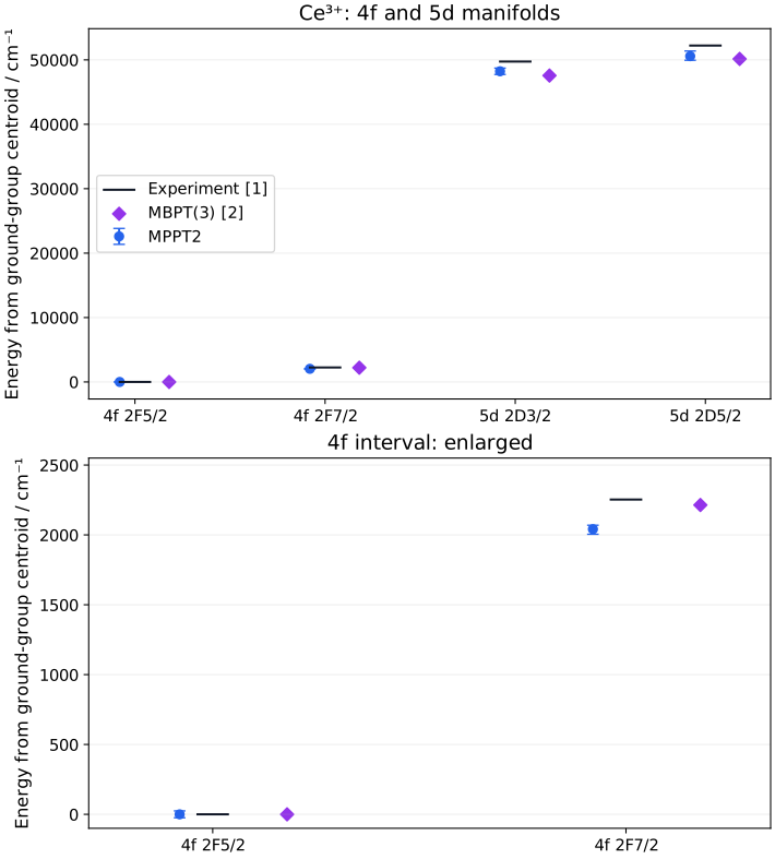
Ce spin–orbit levels compared with experiment and MBPT(3)

Term	MPPT2, cm⁻¹	MBPT(3) [2], cm⁻¹	Experiment [1], cm⁻¹
4f ²F₅/₂	0	0	0
4f ²F₇/₂	2041.19	2214	2253
5d ²D₃/₂	48229.07	47563	49737
5d ²D₅/₂	50575.68	50146	52226

MPPT values are multiplet centroids relative to the ground-group centroid; bars show the minimum–maximum energy range in each group. The MBPT(3) reference uses a relativistic Dirac–Fock/B-spline treatment [2]. The 5d term assignments are approximate: retained states mix J, and the two group widths are 976.02 and 1442.11 cm⁻¹.

Magnetic response and the free-ion limit#

Ce principal and isotropic susceptibilities and effective moment compared with the unsplit free-ion limit

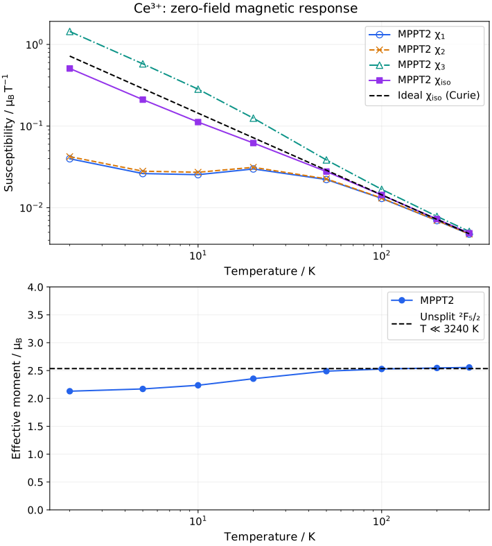
The free-ion reference is the complete 4f ²F₅/₂ multiplet: J=5/2, \(g_J=6/7\) and \(\mu_{\mathrm{eff}}\) = 2.5355 \(\mu_B\). It assumes six degenerate states and temperatures well below the excited ²F₇/₂ manifold, T ≪ 3240 K.

Zero-field quantity	MPPT2	Unsplit ²F₅/₂ reference
\(\mu_{\mathrm{eff}}\) at 2 K, \(\mu_B\)	2.1293	2.5355
\(\mu_{\mathrm{eff}}\) at 300 K, \(\mu_B\)	2.5563	2.5355
\(\chi_{\mathrm{iso}}\) at 300 K, \(\mu_B/\mathrm{T}\)	0.00487714	0.00479796

The computed lowest Kramers pair has g = (0.52301, 0.53533, 4.13614). For that pair alone, the isolated-pair Curie expression gives a low-temperature moment of 2.1017 \(\mu_B\). Its three g components describe two states; \(g_J=6/7\) describes the full six-state multiplet. These are different projections of the moment operator. The response curve includes the other retained pairs and their actual energy separations.

Pr³⁺: multistate 4f² and 4f5d#

Use CAS(2,12) over 4f/5d, averaging 78 singlets and 66 triplets. An initial Pr⁵⁺ singlet RHF calculation prepares the orbitals; casscf.charge: 3 selects the Pr³⁺ target.

The basis is (10s9p9d7f3g2h) → [4s5p5d5f3g2h], with 128 spherical functions and a 28-electron ECP. Selection uses full MOs 10–29, including projected 6s/6p virtuals, and 144 roots. Within this window, the CAS indices are 5–16 and core indices are 1–4.

Input and run#

Pr-df-topk10000.yaml contains the calculation settings; Pr_basis_ecp.basis contains the basis and ECP.

pr/Pr-df-topk10000.yaml#

molecule:
  symmetry: false
  charge: 5
  so: true
  max_memory: 16GB
  atoms:
    - [Pr, 0.0, 0.0, 0.0]
basis:
  Pr: [file, Pr_basis_ecp.basis]
ecp:
  Pr: [file, Pr_basis_ecp.basis]
scf:
  type: rhf
  spin: singlet
  density_fit: true
  auxbasis: null
  conv_tol: 1.0e-12
  omp_num_threads: 8
casscf:
  charge: 3
  spin: triplet
  active_orbitals: 12
  n_active_electrons: 2
  density_fit: true
  auxbasis: null
  conv_tol: 1.0e-10
  conv_tol_grad: 5.0e-5
  max_cycle_micro: 20
  max_cycle_macro: 200
  ah_max_cycle: 50
  ah_start_tol: 2.5
  ah_lindep: 1.0e-15
  ah_conv_tol: 1.0e-14
  ah_level_shift: 0.1
  omp_num_threads: 8
  states_to_average:
    - [singlet, 78]
    - [triplet, 66]
mppt:
  prefix: Pr
  output_hdf5: pyscf_dump.h5
  integral_mode: df
  so_source: scalar
  downstream_nocc: 14
  N_select: 20
  N_start: 10
  avas_labels_analyzis: [Pr 4f, Pr 5d, Pr 6s, Pr 6p]
  avas_labels_virtual: [Pr 6s, Pr 6p]
  generate_projected_virtuals: true
  generate_virtuals_from: 26
  cipsixx:
    enabled: true
    initial_space: cas
    max_selected: 10000
    batch_size: 500
    max_iterations: 40
    max_candidates: 200000
    n_roots: 144
    multi_state: true
    selection_growth: topk
    selection_metric: coefficient
    state_weighting: legacy-taum
    spin_adaptation_closure: spin-projection
    final_diagonalization: always
    cas_orbitals: [5, 6, 7, 8, 9, 10, 11, 12, 13, 14, 15, 16]
    core_orbitals: [1, 2, 3, 4]
    frozen_orbitals: []
    cas_alpha_electrons: 1
    cas_beta_electrons: 1
    omp_num_threads: 8
  diagpt:
    enabled: true
    title: Pr DF-CASSCF topk500 target10000 MPPT2
    integral_space: selected
    omp_num_threads: 8
  heffso:
    enabled: true
    title: Pr DF-CASSCF topk500 target10000 magnetic MPPT2
    iorder: 2
    properties: true
    nvectw: 276
    residual_tolerance: 1.0e-11
    initial_vector_tolerance: 1.0e-10
    omp_num_threads: 8
    magnetic_properties:
      spin_g: 2.0
      fields_tesla: [[0, 0, 0], [0, 0, 1], [0, 0, -1]]
      temperatures_kelvin: [2, 20, 300]
      susceptibility: true

From test_suite/workflows/magnetic/pr/:

pyscf2mppt run Pr-df-topk10000.yaml --output-dir runs/pr10k
caspy-heffso-report --run-dir runs/pr10k --prefix Pr --magnetic

The example contains 4644 physical determinants and 10177 closure rows, with 276 SOC states.

Results versus experiment#

Pr 3H centroids and multiplet widths compared with experiment

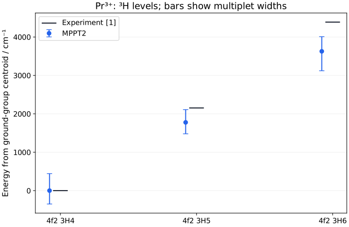
Assigned group	MPPT centroid, cm⁻¹	Experiment [1], cm⁻¹	MPPT width, cm⁻¹
³H₄, states 1–9	0	0	791.43
³H₅, states 10–20	1777.14	2152.09	629.45
³H₆, states 21–33	3628.03	4389.09	887.75

Centroids are relative to the mean of states 1–9; bars show each group’s minimum–maximum range.

Magnetic response and the free-ion limit#

Pr principal and isotropic susceptibilities and effective moment compared with the unsplit free-ion limit

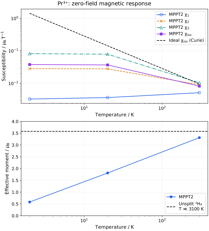
The ³H₄ free-ion reference has J=4, \(g_J=4/5\) and \(\mu_{\mathrm{eff}}\) = 3.5777 \(\mu_B\). Its nine degenerate states give an isotropic Curie susceptibility for T ≪ 3100 K. The calculation retains the level spread shown above, whereas the reference assumes an unsplit ground multiplet.

The strong anisotropy accompanies the 791.43 cm⁻¹ splitting of the nominal ³H₄ multiplet, far above the thermal scale \(k_BT/(hc)=1.39\text{–}208.51\ \mathrm{cm}^{-1}\) over 2–300 K, so unequal populations and inter-level contributions strongly affect the response. Approaching the isotropic free-ion limit calls for a more symmetry-complete, balanced model space and retained-state set, assessed alongside the construction dependence of MPPT; simply selecting more determinants need not reduce the splitting monotonically.

Zero-field quantity at 300 K	MPPT2	Unsplit ³H₄ reference
\(\chi_1\), \(\mu_B/\mathrm{T}\)	0.00513484	0.00955326
\(\chi_2\), \(\mu_B/\mathrm{T}\)	0.00903623	0.00955326
\(\chi_3\), \(\mu_B/\mathrm{T}\)	0.01036976	0.00955326
\(\mu_{\mathrm{eff}}\), \(\mu_B\)	3.3106	3.5777

The computed effective moment rises from 0.5813 \(\mu_B\) at 2 K to 3.3106 \(\mu_B\) at 300 K. Pr³⁺ has an even electron count, so an isolated Kramers-pair g tensor is not the appropriate description of these states.

OH: molecular spin–orbit splitting#

At R(O–H)=0.96966 Å, use uncontracted ANO-RCC with 142 spherical basis functions and the zero-core O08 GRPP from the Gatchina pseudopotential library. SA-CASSCF(7,5) averages the lowest 15 roots in \(M_S=1/2\) over O 2s, σ, \(\pi_x\), \(\pi_y\) and σ*: 12 doublets and 3 quartets in the converged reference. All roots have weight 1/15.

Selection uses full MOs 1–27, including O1s and all nine explicit electrons. In this input, [doublet, 15] fixes \(M_S=1/2\); it does not constrain every root to total spin S=1/2. Exact integrals avoid an auxiliary-basis approximation.

Input and run#

OH-ano-rcc-topk15000.yaml contains the calculation settings; O08.inp is the oxygen GRPP. PySCF reads uncontracted ANO-RCC as unc-ano from its basis library.

oh/OH-ano-rcc-topk15000.yaml#

molecule:
  symmetry: false
  charge: 0
  units: angstrom
  so: true
  max_memory: 16GB
  atoms:
    - [O, 0.0, 0.0, 0.0]
    - [H, 0.0, 0.0, 0.96966]
basis:
  O: [library, unc-ano]
  H: [library, unc-ano]
grpp:
  O: O08.inp
scf:
  type: rohf
  spin: doublet
  initial_guess:
    method: 1e
  density_fit: false
  conv_tol: 1.0e-12
  max_cycle: 150
  omp_num_threads: 8
casscf:
  active_orbitals: 5
  n_active_electrons: 7
  density_fit: false
  avas_labels: [O 2s, O 2p, H 1s]
  avas_basis:
    O: [library, sto-3g]
    H: [library, sto-3g]
  conv_tol: 1.0e-10
  conv_tol_grad: 1.0e-5
  max_cycle_micro: 10
  max_cycle_macro: 200
  omp_num_threads: 8
  states_to_average:
    - [doublet, 15]
mppt:
  prefix: OH
  output_hdf5: pyscf_dump.h5
  integral_mode: exact
  so_source: relativistic
  downstream_nocc: 5
  N_select: 27
  N_start: 1
  avas_labels_analyzis: [O 1s, O 2s, O 2p, H 1s]
  cipsixx:
    enabled: true
    initial_space: cas
    max_selected: 15000
    batch_size: 500
    max_iterations: 60
    max_candidates: 200000
    n_roots: 15
    multi_state: true
    selection_growth: topk
    selection_metric: coefficient
    state_weighting: uniform
    spin_adaptation_closure: spin-projection
    final_diagonalization: always
    cas_orbitals: [2, 3, 4, 5, 6]
    core_orbitals: [1]
    frozen_orbitals: []
    cas_alpha_electrons: 4
    cas_beta_electrons: 3
    omp_num_threads: 8
  diagpt:
    enabled: true
    title: OH ANO-RCC CAS(7,5) SA15 target15000 MPPT2
    integral_space: selected
    omp_num_threads: 8
  heffso:
    enabled: true
    title: OH ANO-RCC CAS(7,5) SA15 magnetic MPPT2
    iorder: 2
    properties: true
    nvectw: 60
    max_basis: 512
    print_level: 2
    residual_tolerance: 1.0e-11
    initial_vector_tolerance: 1.0e-10
    omp_num_threads: 8
    magnetic_properties:
      spin_g: 2.0
      fields_tesla: [[0, 0, 0], [0.1, 0, 0], [-0.1, 0, 0], [0, 0.1, 0], [0, -0.1, 0], [0, 0, 0.1], [0, 0, -0.1], [1, 0, 0], [-1, 0, 0], [0, 1, 0], [0, -1, 0], [0, 0, 1], [0, 0, -1], [5, 0, 0], [-5, 0, 0], [0, 5, 0], [0, -5, 0], [0, 0, 5], [0, 0, -5], [0.2, -0.3, 0.7], [-0.2, 0.3, -0.7]]
      temperatures_kelvin: [2, 5, 10, 20, 50, 100, 200, 300]
      susceptibility: true
      store_field_matrices: true

From test_suite/workflows/magnetic/oh/:

pyscf2mppt run OH-ano-rcc-topk15000.yaml --output-dir runs/oh15k
caspy-heffso-report --run-dir runs/oh15k --prefix OH --magnetic

The 15000-row target gives 8212 physical determinants and 15093 closure rows, with 60 SOC states. Response uses the same 21 fields and eight temperatures as the Ce input.

Experiment, QDNEVPT2 and coupled cluster#

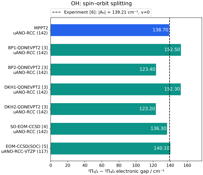
OH spin–orbit splitting compared with QDNEVPT2, coupled cluster and experiment

Method	Splitting, cm⁻¹	Basis	Functions
MPPT2	138.7024	Uncontracted ANO-RCC	142
BP1 / BP2-QDNEVPT2 [3]	152.5 / 123.4	Uncontracted ANO-RCC	142
DKH1 / DKH2-QDNEVPT2 [3]	152.3 / 123.2	Uncontracted ANO-RCC	142
SO-EOM-CCSD [4]	136.3	Uncontracted ANO-RCC	142
EOM-CCSD(SOC) [5]	140.1	Uncontracted ANO-RCC-VTZP	117
Experiment [6], \(\lvert A_0\rvert\) at v=0	139.21	—	—

The MPPT2 Hamiltonian uses the O08 GRPP specified above. Function counts are spherical spatial functions: uncontracted ANO-RCC has 100 on O and 42 on H; uncontracted ANO-RCC-VTZP has 82 on O and 35 on H [7]. Theory values are tabulated in Tables 2–3 of [3], which cites [4] and [5] for the coupled-cluster results.

The QDNEVPT2 reference uses CAS(7,5), 15 equally weighted states and R=0.96966 Å for ANO-RCC or R=0.96970 Å for ANO-RCC-VTZP [3, Tables S1–S2]. The MPPT example matches the S1 geometry, basis and number of equally weighted roots. The SI does not specify their spin decomposition; the MPPT convention is explicit above. Its GRPP Hamiltonian differs from the article’s BP/DKH treatments.

MPPT2 gives a fixed-nuclei electronic splitting, whereas experimental \(A_0\) is the effective spin–orbit constant of the v=0 vibrational level. Quantitative comparison requires at least a bond-length-dependent spin–orbit calculation averaged with the v=0 vibrational probability density. The present comparison is indicative; the 0.51 cm⁻¹ difference alone does not establish sub-cm⁻¹ accuracy.

Magnetic response and the isolated-doublet limit#

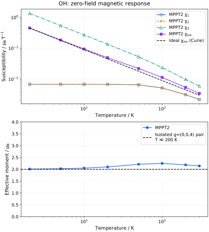
OH principal and isotropic susceptibilities and effective moment compared with an ideal fixed-axis doublet — The transverse susceptibilities \(\chi_1\) and \(\chi_2\) nearly coincide; their curves overlap.#

For an ideal fixed-axis ²Π₃/₂ ground pair, g = (0,0,4): the weak-field response is longitudinal, and the isotropic Curie moment is 2 \(\mu_B\). The molecular axis is z in this input. This is an electronic reference with fixed nuclei, not a rotationally resolved molecular g factor.

Low-temperature quantity	MPPT2	Ideal ²Π₃/₂ pair
\(g_1\)	0.010887	0
\(g_2\)	0.010893	0
\(g_3\)	3.999618	4
\(\mu_{\mathrm{eff}}\) at 2 K, \(\mu_B\) (full response)	2.0099	2

The principal g values describe the lowest pair and give a pair-only Curie moment of 1.9998 \(\mu_B\). The moment row uses the full retained-state response, including inter-state susceptibility contributions. The isolated-pair reference applies for T ≪ 200 K; its dashed extension is a guide only. At 300 K the computed \(\mu_{\mathrm{eff}}\) is 2.1421 \(\mu_B\), where the excited spin–orbit pair is thermally populated and the ground-pair approximation no longer applies.

Calculation outputs#

Each run writes data/<prefix>_heffso_properties.h5 with levels, operators and magnetic response. The Caspy command writes energy and g tables, field-dependent levels, magnetization and susceptibility, plus a magnetic overview in reports/heffso/. See magnetic output for units and the operator model.

References#

[1] Experimental atomic levels. NIST Atomic Spectra Database, Ce IV and Pr IV level tables.

[2] Ce MBPT(3). I. M. Savukov, W. R. Johnson, U. I. Safronova and M. S. Safronova, Phys. Rev. A 67, 042504 (2003), Table I. DOI: 10.1103/PhysRevA.67.042504; arXiv:physics/0210103.

[3] OH QDNEVPT2. R. Majumder and A. Yu. Sokolov, “Consistent Second-Order Treatment of Spin–Orbit Coupling and Dynamic Correlation in Quasidegenerate N-Electron Valence Perturbation Theory,” J. Chem. Theory Comput. (2024), Tables 2–3. DOI: 10.1021/acs.jctc.4c00458; article, Supporting Information, Tables S1–S2.

[4] OH SO-EOM-CCSD. L. Cheng, F. Wang, J. F. Stanton and J. Gauss, “Perturbative treatment of spin-orbit-coupling within spin-free exact two-component theory using equation-of-motion coupled-cluster methods,” J. Chem. Phys. 148, 044108 (2018). DOI: 10.1063/1.5012041.

[5] OH EOM-CCSD(SOC). Z. Cao, Z. Li, F. Wang and W. Liu, “Combining the spin-separated exact two-component relativistic Hamiltonian with the equation-of-motion coupled-cluster method for the treatment of spin–orbit splittings of light and heavy elements,” Phys. Chem. Chem. Phys. 19, 3713–3721 (2017). DOI: 10.1039/C6CP07588F.

[6] OH experimental constants. K. P. Huber and G. Herzberg, Constants of Diatomic Molecules (1979), as compiled in the NIST Chemistry WebBook: A₀=−139.21 cm⁻¹.

[7] Basis definitions. Basis Set Exchange, ANO-RCC and ANO-RCC-VTZP, H and O; spherical function counts obtained by uncontracting their primitive shells.